Digital Optimization & Calculations
| ExperimentSimulation | |
| In progress |
Overview:
Before physically designing my rocket, I use computational simulation software in order to model, test, and optimize rocket aerodynamic and stability performance. This ultimately minimizes structural risk, reduces material waste, and can accurately predict flight characteristics under simulated launch conditions.
Design Process:
The goal is to design a rocket that fulfills certain mission requirements while also being reliable and modular, with constraints being:
- Maximizing apogee for current motor class
- Maintaining rocket stability (within 1-2 calibers)
- Ensure safe descent velocity
- Minimizing drag
- Material quality and surface area in order to improve efficiency
- Capability to carry certain weights (if mission permits)
Phoenix Rocket:
Mission Requirements:
- Be able to carry at least 120 grams of payload for flight computer & camera
- Achieve altitude over 1000ft
- Incorporate 3D printed parts for first time
These were the steps and changes ultimately made during the digital design of the rocket, will go more in depth later on.
1. Baseline Model
- Standard body tube + ogive nose cone
- Three-fin configuration
- Initial motor test
2. Stability Adjustment
- Increased fin surface area
- Modified sweep angle
- Adjusted nose mass distribution
3. Drag Optimization
- Reduced fin thickness
- Refined root chord length
- Evaluated altitude impact of added stability components
To solve for rocket stability caliber, essentially meaning the rocket’s ability to correct itself during flight, can be represented with the equation below. CP stands for the Center of Pressure, or essentially where the sum of aerodynamic forces on the rocket react. Next is CG, or the Center of Gravity, is the location where the total force of gravity appears to act, and where the rocket is balanced in all directions. Lastly, D, is simply the diameter of the rocket.
Initial:
Initial simulations proved that the rocket was initially only capable of reaching 900ft with 65.26 grams of payload. In order to correct rocket characteristics in order to fit mission requirements, reducing the rocket size from 57” to 45” was necessary, combined with smaller fins reduced from around 11” in length and 4” in height to 7” in length and 2” in height, while still maintaining proper stability.
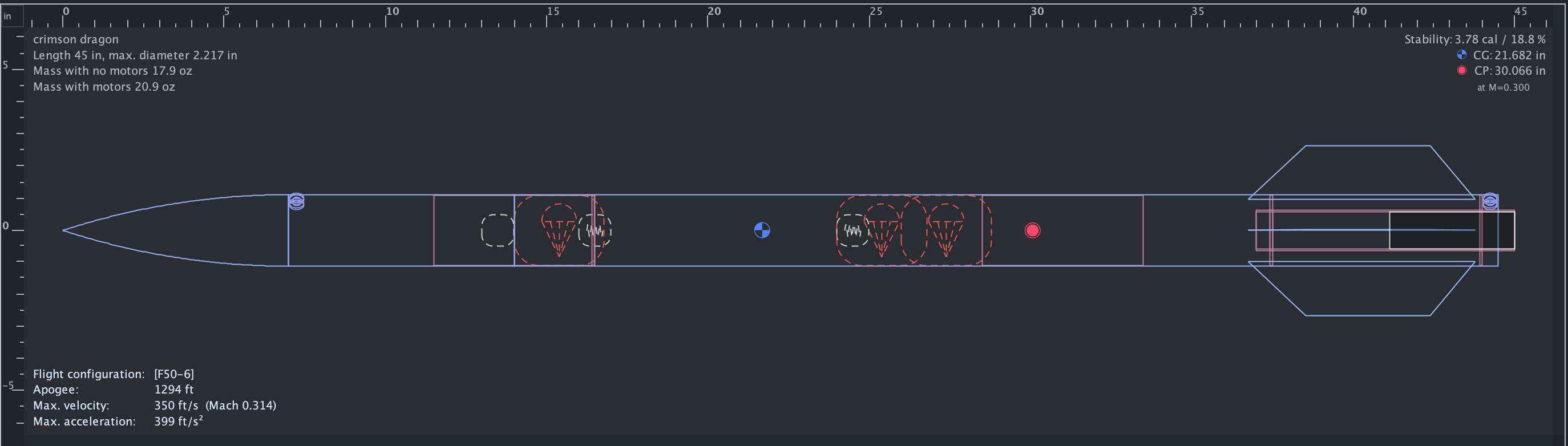
However, as seen here, even with a 120 gram payload mass and powerful motor, the rocket still manages a 3.78 stability caliber, exceeding the 1-2 caliber stability range seen before. After looking through individual mass components, I discovered that the nose cone weighed 161.39 grams instead of 48 grams!
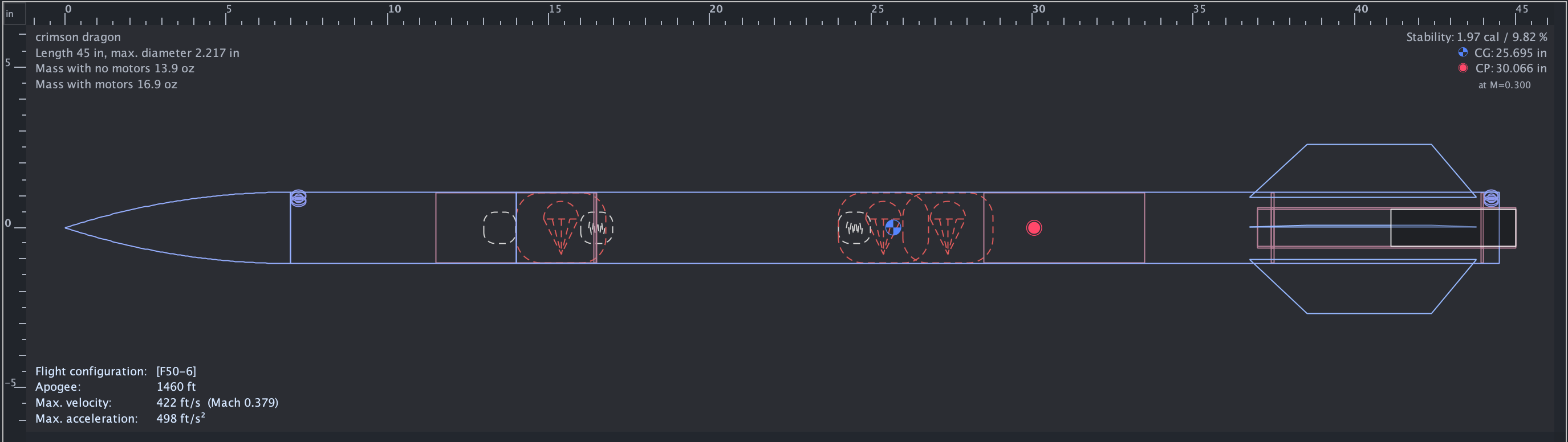
Ultimately resulting in a 166ft gain and a 1.97 caliber, allowing the rocket to be stable and “calibrate” itself during flight from wind changes in speed and direction.
Performance Metrics:
Core flight data: CONFIGURATION: (F50-6)
| Predicted Apogee | 1459.72 ft |
| Maximum Velocity | 285.97 mph |
| Peak Acceleration | 15.48 G |
| Burn time | 1.42 sec |
| Time to apogee (max height) | 7.74 sec |
| Drag coefficient | N/A Requires CFD Software (will later be published) |
| Descent rate under parachute | 6.69 mph |
| Flight time (Total) | 175 sec |
Analysis:
Apogee
The final configuration achieved a predicted apogee of around 1460ft. While higher altitudes were attainable using larger fins or lighter construction, those changes reduced structural robustness and stability margin. The selected configuration balanced altitude optimization with flight reliability with the mission objective of carrying a 120g payload as well. However, since this is not a competition rocket and is purely made for scientific/videography purposes, the maximum apogee is ultimately irrelevant compared to flight stability or speed.
Velocity
Acceleration
Drag Coefficient
Equations used:
Drag Equation
Thrust to Weight Ratio
Rocket Thrust Equation
This formula is used to calculate the thrust of a rocket.
While the full thrust equation provides a theoretical framework for understanding rocket propulsion, flight simulations were ultimately based on manufacturer thrust curve data. Because commercial motors are proven and tested, their published performance already incorporates real combustion and nozzle effects. Using this measured data improved modeling reliability and reduced dependence on assumed thermodynamic parameters.
F: Thrust force (Newtons)
ṁ: Propellant mass flow rate
: Exit velocity of exhaust gasses
: Pressure of the exhaust gas at nozzle exit
: Ambient atmospheric pressure
: Cross-sectional area of nozzle exit
- In our case, F would be simply represented as 50 newtons, as the “50” in “F50” simply indicates the thrust force in newtons.
- Next, ṁ is calculated through the equation of:
represents the total mass of fuel and oxidizer consumed, and represents the total time that the engine is firing. So, with 38g of total fuel, and with a 1.4 second burn time, our ṁ would be 0.027 kg/s. So, the motor ejects around 0.027 kg of mass every second.
💡However, this assumes that the rocket engine fires at 0.027 kg/s until all of the propellant is gone. In reality, this will shift due to manufacturing conditions or environmental factors, but for the sake of this equation, we assume that 0.027 kg/s is constant.
- is calculated through the equation of:
With the variables each representing:
ṁ: Mass flow rate
: Exhaust velocity
So, our mass flow rate of our engine (found above) would be around 0.027kg/s, and F would simply be 50. So simplifying the equation to look like this:
We get to equal around 1851.8 m/s for our final exhaust velocity.
💡Although exhaust velocity can be derived using the isentropic nozzle expansion theory, this approach requires precise knowledge of chamber pressure, combustion temperature, and exhaust gas properties — parameters not publicly available for commercial F50-6 motors. Additionally, solid composite motors produce two-phase exhaust flow, violating the ideal gas assumptions of isentropic modeling. Instead, I relied on experimentally measured thrust curves and total impulse data, ensuring that performance estimates were grounded in early testing rather than thermodynamic assumptions.
- To solve for , you first have to solve for
Multistage Performance